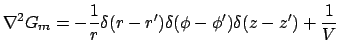
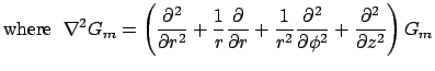
The GF stated below contains a double summation with eigenfunctions ![]() norms
norms ![]() and
and ![]() , eigenvalues
, eigenvalues ![]() and kernel function
and kernel function
![]() , as follows:
, as follows:
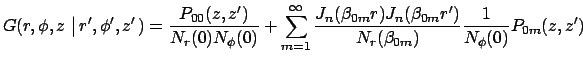 |
(4) | ||
![$\displaystyle + \sum_{n=1}^{\infty }\sum^{\infty}_{m=1}
\frac{ J_n(\beta_{nm}r)...
...a_{nm})}
\frac{\cos[n(\phi - \phi^{\prime})]}{N_{\phi}(n)}
P_{nm}(z,z^{\prime})$](img50.png) |
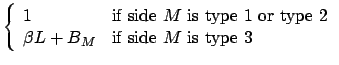
| Boundary at | |||
| Case | for |
for |
|
| R01 |
|
same as |
|
| R02 |
|
|
|
| R03 |
|
|
same as |
| Case | eigencondition |
| R01 |
|
| R02 |
|
| R03 |
|
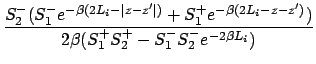
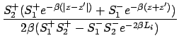
Kernel functions
The kernel function
![]() must satisfy
must satisfy
| (5) |
 |
(6) | ||
 |
 |
(7) | ||
 |
(8) |
The expression for ![]() in Eq. (7) is symmetric if
in Eq. (7) is symmetric if ![]() and
and ![]() are interchanged and covers several combinations of boundary conditions
provided
are interchanged and covers several combinations of boundary conditions
provided ![]() . The special case of
. The special case of ![]() is discussed below.
is discussed below.
Kernel function with ![]()
If the ![]() face of the cylinder is of type 2, then the
zero eigenvalue exists. In this case the
kernel function must satisfy
face of the cylinder is of type 2, then the
zero eigenvalue exists. In this case the
kernel function must satisfy
| (9) |
| Case |
|
| Z11 |
|
| Z12 | |
| Z13 |
|
| Z21 | |
| Z22 |
((
|
| Z23 |
|
| Z31 |
|
| Z32 |
|
| Z33 |
|
|
|
Modified GF for Case R02![]() Z22
Z22
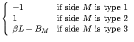
A very special condition occurs if the cylinder's entire boundary
has type 2 (Neumann) conditions. In this case the ordinary Green's
function, defined above, does not exist.
However the GF method can be used if we define a modified GF,
following Barton (Elements of Green's Functions and Propagation,
Oxford University Press, 1989), as follows:
 |
(10) | ||
 |
|||
| (11) |
Modified Green's function ![]() may be used to find temperature with
the Green's function solution equation, Eq. (2), with the following additional
constraints: the sum of the heat passing through the boundaries must
be equal to the total amount of heat introduced by volume energy
generation
may be used to find temperature with
the Green's function solution equation, Eq. (2), with the following additional
constraints: the sum of the heat passing through the boundaries must
be equal to the total amount of heat introduced by volume energy
generation ![]() ; and, since the spatial average temperature of the body
computed from
; and, since the spatial average temperature of the body
computed from ![]() is zero, the average temperature in the body
must be supplied as part of the input data to the problem. Further
discussion and numerical examples of steady heat conduction in the cylinder
may be found in a paper by Cole (K.D. Cole, "Fast converging series for
heat conduction in the circular cylinder," J. of Engineering Mathematics,
vol. 49, pp. 217-232, 2004).
is zero, the average temperature in the body
must be supplied as part of the input data to the problem. Further
discussion and numerical examples of steady heat conduction in the cylinder
may be found in a paper by Cole (K.D. Cole, "Fast converging series for
heat conduction in the circular cylinder," J. of Engineering Mathematics,
vol. 49, pp. 217-232, 2004).