Next: HEAT EQUATION EXAMPLE
Up: What is Green's Function
Previous: What is Green's Function
Consider the steady temperature  in a fin of uniform cross section,
which satisfies the following second order, linear, differential equation:
in a fin of uniform cross section,
which satisfies the following second order, linear, differential equation:
Figure:
Geometry for fin example.
![\includegraphics[height=4cm]{whatisG_fin_example.eps}](img3.png) |
Here 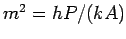 where
where  is the heat transfer
coefficient (
is the heat transfer
coefficient ( ),
),  is the fin
perimeter (meters),
is the fin
perimeter (meters),  is the cross section area of the fin (meters squared),
and
is the cross section area of the fin (meters squared),
and  is the thermal conductivity (
 ). Quantity
  describes heat loss by convection to a fluid at temperature zero
from the sides of the
fin (if the fluid temperature is at some
describes heat loss by convection to a fluid at temperature zero
from the sides of the
fin (if the fluid temperature is at some
 you can
always define
you can
always define
 to reset the fluid temperature to
zero). Refer to the figure for the geometry.
Term
to reset the fluid temperature to
zero). Refer to the figure for the geometry.
Term  represents
volume energy generation within the fin (such as by electric heating or
chemical reaction). The boundary conditions at the
ends of the fin may be of several types, however consider the following
specific boundary conditions:
represents
volume energy generation within the fin (such as by electric heating or
chemical reaction). The boundary conditions at the
ends of the fin may be of several types, however consider the following
specific boundary conditions:
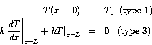
The boundary at  is fixed at specified temperature
  and
the boundary at
and
the boundary at  sees heat loss by convection.
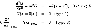
The temperature solution will be solved in terms of the Green's
function, which is the response of the fin to a point source of heat.
The GF for the above fin satisfies the following equations:
Note that the above equations are similar to the temperature problem, except
the energy generation term is replaced by a Dirac delta function and the
boundary conditions are homogeneous. Most importantly, the boundary
conditions must be of the same type as the specific temperature
problem of
interest. The Green's function
 represents the heat transfer
response at observation point
represents the heat transfer
response at observation point  to an infinitesimal heat source located
at point
to an infinitesimal heat source located
at point  .
.
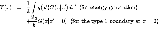
The temperature solution is constructed from a suitable distribution of the GF
within the body so as to reproduce the heating conditions. In this example,
the temperature in
the fin is given by:
The temperature solution contains an additive term for each non-homogeneous
heating effect, in this case internal generation  and boundary
temperature . There is no additive term needed for cooling effect
at because this condition is homogeneous (temperature
and boundary
temperature . There is no additive term needed for cooling effect
at because this condition is homogeneous (temperature  appears in
every term of the boundary condition). For a further discussion of steady
heat conduction, see ``Green's function solution equation''.
appears in
every term of the boundary condition). For a further discussion of steady
heat conduction, see ``Green's function solution equation''.
Next: HEAT EQUATION EXAMPLE
Up: What is Green's Function
Previous: What is Green's Function
2004-01-21