Heat Equation, 1-D Rectangular Case.

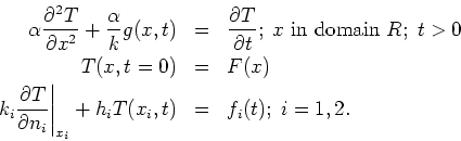
Consider the following boundary-value problem for temperature in a 1-D body in rectangular coordinates:

$$\begin{eqnarray*} \alpha \frac{\partial ^{2}T}{\partial x^{2}}+\frac{\alpha }{k}... ... n_{i}}\right\vert _{x_{i}}+h_{i}T(x_{i},t) &=&f_{i}(t);\;i=1,2. \end{eqnarray*}$$

Note that $n_{i}$ is the outward normal on boundary $i$. The convective (type 3) boundary conditions are specified on boundaries $i=1$ and $i=2$. Boundary conditions of type 1 or 2 are also included by this relationship by taking $k_{i}=0$ or $h_{i}=0$, respectively, on boundaries $i=1$ or $i=2$.

The Green's Function Solution Equation for temperature $T(x,t)$ is given by:

$$\begin{eqnarray*} T(x,t) &=&\int_{x^{\prime }}G(x,t \left\vert x^{\prime },0\... ...{x^{\prime }=x_{i}}% \right] \; \mbox{(for b.c. of type 1 only)} \end{eqnarray*}$$

The spatial integrals should be evaluated over the whole body, for example, on $(0<x^{\prime }<L)$ for a plate, or over $(0<x^{\prime }<\infty )$ for a semi-infinte body. The sumations in the boundary condition terms represent at most two boundaries.

The same GF appears in each integral term, evaluated at the source location $% (x^{\prime },\tau )$ appropriate for that integral term. For example, in the initial-condition integral the GF is evaluated at $\tau =0$; in a boundary-condition integral the GF is evaluated at $x^{\prime }=x_{i}$,